
How the Archive Calculates Values in the Planetary Systems Composite Parameters Table
The Planetary Systems Composite Parameters (PSCompPars) table uses data and empirically derived relationships from the literature to create a near-comprehensive database of key physical parameters for all confirmed exoplanets and their host stars. While the full set of parameters for a given system may not be internally consistent, as parameter values are often drawn from multiple references, this table allows users to explore overarching demographic properties. Here, we describe the underlying logic and formulae used to generate this table.
Table Population Using Empirical Data from the Literature
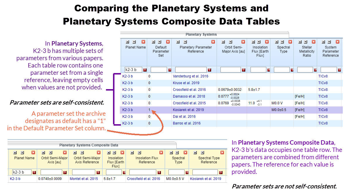
The population of the Planetary Systems Composite Parameters Table differs in one significant way from that of the Planetary Systems (PS) table. In the PS table, all ingested planetary solutions are available with each row representing one reference per solution for each planet. As such, any one planet may have multiple entries in the table, but each row only represents one self-consistent solution as published in the original reference. However, any one row may have many parameters with no values, as those values were not published with the self-consistent set of planetary and stellar parameters.
By contrast, the goal of the PSCompPars table is to provide users with a table that is as complete as possible with a single row of data per planet. This indicates the PSCompPars table will necessarily include parameters from a variety of references for a given planet, indicating the set of reported parameter values may not be internally or physically self-consistent. But, unlike the PS table, there will be only one row per planet in the PSCompPars table.
The following info graphic illustrates the differences between the Planetary Systems and Planetary Systems Composite Parameters tables: (Click to enlarge)
General Algorithm for Selection of Empirical Parameter Values
The decision tree for populating a given parameter for a given planet in the Planetary Systems Composite Parameters table with a value from the literature is as follows:
If, for a given parameter for a given planet...
- ...a value exists and that value is attributed to the default reference in the Planetary Systems table, use that value.
- ...there does not exist a value attributed to the default reference in the Planetary Systems table, use the value for that parameter that has the smallest absolute uncertainty. In the case of asymmetric uncertainties, average the uncertainties to estimate the absolute uncertainty.
- ...there does not exist a value attributed to the default reference in the Planetary Systems table and multiple parameter values have equal absolute uncertainties, use the parameter value from the most recent publication.
Table Population Using Physically Motivated Mathematical Relationships
Here we describe and explicitly list the formulae used to calculate values for certain planetary or stellar parameters, using the empirically determined values of other parameters reported in the Planetary Systems Composite Parameters table as input.
But first, a few notes about our parameter value calculations:
- We do not calculate a given parameter value if at least one of the input parameter values required for the calculation is a limit and not a central value.
- We do not report uncertainties for any parameter value that has been calculated.
- The associated reference column for a parameter value that has been calculated reads "Calculated Value," as it is not tied to a literature reference.
Angular Separation $\rho_{\mathrm{sep}}$
For planets for which the archive has values for both distance to the system, $d$, and orbital semi-major axis, $a$, but not an angular separation, $\rho_{\mathrm{sep}}$, we calculate the angular separation as $$\rho_{\mathrm{sep}} = a/d.$$
Here, $\rho_{\mathrm{sep}}$ represents the angle subtended by an arc the length of the semi-major axis in the plane of the sky at the distance of the system. In the case of a circular orbit, this is equal to both the angular projected semi-major axis and the maximum angular separation of the planet from its host star.
Note that values from the literature may represent closely related but distinct physical quantities—for example, the measured angular separation at a given epoch (which may vary significantly over time), or the maximum possible projected angular separation, which for eccentric orbits depends on the orientation of the orbit and may not be the same as the value that we calculate. If in doubt, refer to the original data source for further information.
Planet Radius $R_{p}$
For planets that do have an empirically determined value for the planet mass $M_{p}$ but do not have an empirically determined value for the planet radius $R_{p}$, regardless of whether the planet has an empirically determined planet density $\rho_{p}$, we invoke the mass-radius relation of Chen & Kipping (2017) to derive the planet radius $R_{p}$. Chen & Kipping (2017) define a four-term piecewise power law function that spans the masses of all planetary objects in the NASA Exoplanet Archive. The form for deriving a planet radius $R_{p}$, given a planet mass $M_{p}$, is the following:
$$ \mathcal{R} = \mathcal{C} + \mathcal{M} \times \mathcal{S},~{\rm where} $$ $\mathcal{R}$ = log$_{10}$($R_{p}$/$R_{\oplus}$), $\mathcal{C}$ = a constant term (in log$_{10}$ units), $\mathcal{M}$ = log$_{10}$($M_{p}$/$M_{\oplus}$), $\mathcal{S}$ = the slope of the power-law relation, $R_{\oplus}$ represents the radius of the Earth, and $M_{\oplus}$ represents the mass of the Earth. We use the following parameters, which are provided in their Table 2 (or derived thereof), to compute a planet radius $R_{p}$ given an input, empirically determined planet mass $M_{p}$: $$ \{\mathcal{C};~\mathcal{S}\} = \begin{cases} \{0.00346; \hspace{3.5mm} 0.2790\} & \text{if}~~~M_{p} < 2.04 M_{\oplus} \\ \{-0.0925; \hspace{2.5mm} 0.589\} & \text{if}~~~2.04 \le M_{p} / M_{\oplus} < 132 \\ \{1.25; \hspace{6.2mm} -0.044\} & \text{if}~~~132 \le M_{p} / M_{\oplus} < 26600 \\ \{-2.85; \hspace{6.2mm} 0.881\} & \text{if}~~~M_{p} \ge 26600 M_{\oplus}. \end{cases} $$Planet Mass $M_{p}$
For planets that do have an empirically determined value for the planet radius $R_{p}$ but do not have an empirically determined value for the planet mass $M_{p}$, regardless of whether the planet has an empirically determined planet density $\rho_{p}$, we rearrange the form of the mass-radius relation presented in Chen & Kipping (2017) (and reproduced above) to provide a radius-mass relation. The form for deriving a planet mass $M_{p}$, given a planet radius $R_{p}$, is the following:
$$ \mathcal{M} = (\mathcal{R} - \mathcal{C}) / \mathcal{S}. $$However, it is crucial to note that, since the third term of the mass-radius relation has a negative slope (i.e., $\mathcal{S} < 0$), there exists a regime of planet radius $R_{p}$ for which a given planet radius $R_{p}$ does not uniquely map into a single planet mass $M_{p}$. This inherently degenerate regime spans approximately ${11.1 \le R_{p} / R_{\oplus} \le 14.3}$. We thus abstain from calculating a planet mass $M_{p}$ in this regime, which spans multiple orders of magnitude (in planet mass $M_{p}$). The resulting piecewise function is thus:
$$ \{\mathcal{C};~\mathcal{S}\} = \begin{cases} \{0.00346; \hspace{3.5mm} 0.2790\} & \text{if}~~~R_{p} < 1.23 R_{\oplus} \\ \{-0.0925; \hspace{2.5mm} 0.589\} & \text{if}~~~1.23 \le R_{p} / R_{\oplus} < 11.1 \\ \{-2.85; \hspace{6.2mm} 0.881\} & \text{if}~~~R_{p} \ge 14.3 R_{\oplus}. \end{cases} $$Planet Density $\rho_{p}$
For planets for which the archive has both the planetary radius $R_{p}$ and the planetary mass $M_{p}$, but for which the archive does not have a planet density $\rho_{p}$, the density is calculated from the mass and volume of the planet, assuming the planet is a sphere. The explicit functional form is:
$$ \rho_{p} = 3M_{p} / (4\pi R_{p}^{3}). $$
Stellar Luminosity $L_{*}$
For host stars for which the archive has both the stellar radius $R_{*}$ and the stellar effective temperature $T_{\rm eff}$, but for which the archive does not have a stellar luminosity $L_{*}$, we use the Stefan-Boltzmann Law. The explicit functional form is:
$$ L_{*} = 4\pi R_{*}^{2} \sigma T_{\rm eff}^{4}. $$
References
Chen, J., & Kipping, D. 2017, ApJ, 834, 17
See Also:
- Developing a More Integrated NASA Exoplanet Archive: How the archive's data tables and services are changing, and when.
- Archive 2.0 Release Notes
- Planetary Systems Composite Parameters Interactive Table: The web version of the data table.
- About the Planetary Systems Composite Parameter Table: How this table is built and used.
- Exoplanet Criteria: The archive's policy on including and excluding planets.
- Planetary Systems and Planetary Systems Composite Parameters Table Definitions: A detailed list and description of each parameter in the Planetary Systems and Planetary Systems Composite Parameters tables.
- Table Access Protocol (TAP) User Guide: Build a a query to automate data downloads from the PS and PSCompPars tables.
Last updated: 2 May 2024


![]()
![]()